86372559

You read ‘Dai Park Textbook’ in category ‘Papers’ When it turns out you prepared less than the demand for the period, the backorder cost b per every missed sale will occur. The amount of missed sales cannot be negative, so it can be represented by max(D? y, 0) or (D? y)+ . When it turns out you prepared more, the quantity of left-over items also cannot go negative, so it can be expressed as max(y? D, 0) or (y? D)+ .

In this way of thinking, we have the following formula. Pro? t =Revenue? Cost =Revenue? Ordering cost? Holding cost? Backorder cost =p(D? y)? (cf + ycv )? h(y? D)+? b(D? y)+ (1. 1) How about the second interpretation of pro? t? You earn p? cv dollars every time you sell a paper. For left-over items, you lose the price you bought in addition to the holding cost per paper, i. e. cv + h. When the demand is higher than what you prepared, you lose b backorder cost. Of course, you also have to pay the? xed ordering cost cf as well when you place an order. With this logic, we have the following pro? t function. Pro? t =Earning?

Loss =(p? cv )(D? y)? (cv + h)(y? D)+? b(D? y)+? cf (1. 2) 1. 1. PROFIT MAXIMIZATION 7 Since we used two di? erent approaches to model the same pro? t function, (1. 1) and (1. 2) should be equivalent. Comparing the two equations, you will also notice that (D? y) + (y? D)+ = y. Now our quest boils down to maximizing the pro? t function. However, (1. 1) and (1. 2) contain a random element, the demand D. We cannot maximize a function of random element if we allow the randomness to remain in our objective function. One day demand can be very high. Another day it is also possible nobody wants to buy a single paper. We have to? ure out how to get rid of this randomness from our objective function. Let us denote pro? t for the nth period by gn for further discussion. Theorem 1. 1 (Strong Law of Large Numbers). Pr g1 + g2 + g3 + + gn = E[g1 ] n>? n lim =1 The long-run average pro? t converges to the expected pro? t for a single period with probability 1. Based on Theorem 1. 1, we can change our objective function from just pro? t to expected pro? t. In other words, by maximizing the expected pro? t, it is guaranteed that the long-run average pro? t is maximized because of Theorem 1. 1. Theorem 1. 1 is the foundational assumption for the entire course.

When we will talk about the long-run average something, it involves Theorem 1. 1 in most cases. Taking expectations, we obtain the following equations corresponding to (1. 1) and (1. 2). E[g(D, y)] =pE[D? y]? (cf + ycv )? hE[(y? D)+ ]? bE[(D? y)+ ] =(p? cv )E[D? y]? (cv + h)E[(y? D)+ ]? bE[(D? y)+ ]? cf (1. 4) (1. 3) Since (1. 3) and (1. 4) are equivalent, we can choose either one of them for further discussion and (1. 4) will be used. Before moving on, it is important for you to understand what E[D? y], E[(y? D)+ ], E[(D? y)+ ] are and how to compute them. Example 1. 1. Compute E[D? 18], E[(18? D)+ ], E[(D? 8)+ ] for the demand having the following distributions. 1. D is a discrete random variable. Probability mass function (pmf) is as follows. d PrD = d 10 1 4 15 1 8 20 1 8 25 1 4 30 1 4 Answer: For a discrete random variable, you? rst compute D? 18, (18? D)+ , (D? 18)+ for each of possible D values. 8 d CHAPTER 1. NEWSVENDOR PROBLEM 10 1 4 15 1 8 20 1 8 25 1 4 30 1 4 PrD = d D? 18 (18? D)+ (D? 18)+ 10 8 0 15 3 0 18 0 2 18 0 7 18 0 12 Then, you take the weighted average using corresponding PrD = d for each possible D. 1 1 1 1 1 125 (10) + (15) + (18) + (18) + (18) = 4 8 8 4 4 8 1 1 1 1 1 19 + E[(18?

D) ] = (8) + (3) + (0) + (0) + (0) = 4 8 8 4 4 8 1 1 1 1 1 + E[(D? 18) ] = (0) + (0) + (2) + (7) + (12) = 5 4 8 8 4 4 E[D? 18] = 2. D is a continuous random variable following uniform distribution between 10 and 30, i. e. D? Uniform(10, 30). Answer: Computing expectation of continuous random variable involves integration. A continuous random variable has probability density function usually denoted by f . This will be also needed to compute the expectation. In this case, fD (x) = 1 20 , 0, if x? [10, 30] otherwise Using this information, compute the expectations directly by integration.? E[D? 18] =? 30 (x? 18)fD (x)dx (x? 18) 10 18 = = 10 18 1 dx 20 1 20 dx + 30 (x? 18) x 10 dx + 18 30 (x? 18) 1 20 dx 1 20 dx = = x2 40 1 20 + 18 x=18 x=10 18x 20 18 x=30 x=18 The key idea is to remove the? operator that we cannot handle by separating the integration interval into two. The other two expectations can 1. 1. PROFIT MAXIMIZATION be computed in a similar way. 9? E[(18? D)+ ] =? 30 (18? x)+ fD (x)dx (18? x)+ 10 18 = = 10 18 1 dx 20 1 20 1 20 +0 30 (18? x)+ (18? x) 10 x2 2 x=18 dx + 18 30 (18? x)+ 0 18 1 20 dx = dx + 1 20 dx 18x? = 20 x=10? E[(D? 18)+ ] =? 30 (18? x)+ fD (x)dx (x? 8)+ 10 18 = = 10 18 1 dx 20 1 20 30 (x? 18)+ 0 10 x2 2 dx + 18 30 (x? 18)+ 1 20 dx 1 20 dx = =0 + 1 20 dx + 18 x=30 (x? 18)? 18x 20 x=18 Now that we have learned how to compute E[D? y], E[(y? D)+ ], E[(D? y)+ ], we have acquired the basic toolkit to obtain the order quantity that maximizes the expected pro? t. First of all, we need to turn these expectations of the pro? t function formula (1. 4) into integration forms. For now, assume that the demand is a nonnegative continuous random variable. 10 CHAPTER 1. NEWSVENDOR PROBLEM E[g(D, y)] =(p? cv )E[D? y]? (cv + h)E[(y? D)+ ]? bE[(D? y)+ ]? f? =(p? cv ) 0 (x? y)fD (x)dx? (cv + h) 0? (y? x)+ fD (x)dx?b 0 (x? y)+ fD (x)dx? cf y? =(p? cv ) 0 xfD (x)dx + y y yfD (x)dx? (cv + h) 0? (y? x)fD (x)dx?b y (x? y)fD (x)dx? cf y y =(p? cv ) 0 xfD (x)dx + y 1? 0 y y fD (x)dx xfD (x)dx? (cv + h) y 0 y fD (x)dx? 0 y? b E[D]? 0 xfD (x)dx? y 1? 0 fD (x)dx? cf (1. 5) There can be many ways to obtain the maximum point of a function. Here we will take the derivative of (1. 5) and set it to zero. y that makes the derivative equal to zero will make E[g(D, y)] either maximized or minimized depending on the second derivative.

For now, assume that such y will maximize E[g(D, y)]. We will check this later. Taking the derivative of (1. 5) will involve di? erentiating an integral. Let us review an important result from Calculus. Theorem 1. 2 (Fundamental Theorem of Calculus). For a function y H(y) = c h(x)dx, we have H (y) = h(y), where c is a constant. Theorem 1. 2 can be translated as follows for our case. y d xfD (x)dx =yfD (y) dy 0 y d fD (x)dx =fD (y) dy 0 (1. 6) (1. 7) Also remember the relationship between cdf and pdf of a continuous random variable. y FD (y) =? fD (x)dx (1. 8) 1. 1. PROFIT MAXIMIZATION Use (1. 6), (1. 7), (1. ) to take the derivative of (1. 5). d E[g(D, y)] =(p? cv ) (yfD (y) + 1? FD (y)? yfD (y)) dy? (cv + h) (FD (y) + yfD (y)? yfD (y))? b (? yfD (y)? 1 + FD (y) + yfD (y)) =(p + b? cv )(1? FD (y))? (cv + h)FD (y) =(p + b? cv )? (p + b + h)FD (y) = 0 If we di? erentiate (1. 9) one more time to obtain the second derivative, d2 E[g(D, y)] =? (p + b + h)fD (y) dy 2 11 (1. 9) which is always nonpositive because p, b, h, fD (y)? 0. Hence, taking the derivative and setting it to zero will give us the maximum point not the minimum point. Therefore, we obtain the following result. Theorem 1. 3 (Optimal Order Quantity).

The optimal order quantity y? is the smallest y such that FD (y) = p + b? cv? 1 or y = FD p+b+h p + b? cv p+b+h . for continuous demand D. Looking at Theorem 1. 3, it provides the following intuitions. ¢ Fixed cost cf does not a? ect the optimal quantity you need to order. ¢ If you can procure items for free and there is no holding cost, you will prepare as many as you can. ¢ If b h, b cv , you will also prepare as many as you can. ¢ If the buying cost is almost as same as the selling price plus backorder cost, i. e. cv? p + b, you will prepare nothing. You will prepare only upon you receive an order.

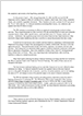
Example 1. 2. Suppose p = 10, cf = 100, cv = 5, h = 2, b = 3, D? Uniform(10, 30). How many should you order for every period to maximize your long-run average pro? t? Answer: First of all, we need to compute the criterion value. p + b? cv 10 + 3? 5 8 = = p+b+h 10 + 3 + 2 15 Then, we will look up the smallest y value that makes FD (y) = 8/15. 12 1 CHAPTER 1. NEWSVENDOR PROBLEM CDF 0. 5 0 0 5 10 15 20 25 30 35 40 D Therefore, we can conclude that the optimal order quantity 8 62 = units. 15 3 Although we derived the optimal order quantity solution for the continuous demand case, Theorem 1. applies to the discrete demand case as well. I will? ll in the derivation for discrete case later. y? = 10 + 20 Example 1. 3. Suppose p = 10, cf = 100, cv = 5, h = 2, b = 3. Now, D is a discrete random variable having the following pmf. d PrD = d 10 1 4 15 1 8 20 1 8 25 1 4 30 1 4 What is the optimal order quantity for every period? Answer: We will use the same value 8/15 from the previous example and look up the smallest y that makes FD (y) = 8/15. We start with y = 10. 1 4 1 1 3 FD (15) = + = 4 8 8 1 1 1 1 FD (20) = + + = 4 8 8 2 1 1 1 1 3 FD (25) = + + + = 4 8 8 4 4? Hence, the optimal order quantity y = 25 units.

FD (10) = 8 15 8 &lt, 15 8 &lt, 15 8? 15 &lt, 1. 2 Cost Minimization Suppose you are a production manager of a large company in charge of operating manufacturing lines. You are expected to run the factory to minimize the cost. Revenue is another person’s responsibility, so all you care is the cost. To model the cost of factory operation, let us set up variables in a slightly di? erent way. 1. 2. COST MINIMIZATION 13 ¢ Understock cost (cu ): It occurs when your production is not su? cient to meet the market demand. ¢ Overstock cost (co ): It occurs when you produce more than the market demand.

In this case, you may have to rent a space to store the excess items. ¢ Unit production cost (cv ): It is the cost you should pay whenever you manufacture one unit of products. Material cost is one of this category. ¢ Fixed operating cost (cf ): It is the cost you should pay whenever you decide to start running the factory. As in the pro? t maximization case, the formula for cost expressed in terms of cu , co , cv , cf should be developed. Given random demand D, we have the following equation. Cost =Manufacturing Cost + Cost associated with Understock Risk + Cost associated with Overstock Risk =(cf + ycv ) + cu (D? )+ + co (y? D)+ (1. 10) (1. 10) obviously also contains randomness from D. We cannot minimize a random objective itself. Instead, based on Theorem 1. 1, we will minimize expected cost then the long-run average cost will be also guaranteed to be minimized. Hence, (1. 10) will be transformed into the following. E[Cost] =(cf + ycv ) + cu E[(D? y)+ ] + co E[(y? D)+ ]? =(cf + ycv ) + cu 0? (x? y)+ fD (x)dx + co 0 y (y? x)+ fD (x)dx (y? x)fD (x)dx (1. 11) 0 =(cf + ycv ) + cu y (x? y)fD (x)dx + co Again, we will take the derivative of (1. 11) and set it to zero to obtain y that makes E[Cost] minimized.

We will verify the second derivative is positive in this case. Let g here denote the cost function and use Theorem 1. 2 to take the derivative of integrals. d E[g(D, y)] =cv + cu (? yfD (y)? 1 + FD (y) + yfD (y)) dy + co (FD (y) + yfD (y)? yfD (y)) =cv + cu (FD (y)? 1) + co FD (y)? (1. 12) The optimal production quantity y is obtained by setting (1. 12) to be zero. Theorem 1. 4 (Optimal Production Quantity). The optimal production quantity that minimizes the long-run average cost is the smallest y such that FD (y) = cu? cv or y = F? 1 cu + co cu? cv cu + co . 14 CHAPTER 1. NEWSVENDOR PROBLEM Theorem 1. can be also applied to discrete demand. Several intuitions can be obtained from Theorem 1. 4. ¢ Fixed cost (cf ) again does not a? ect the optimal production quantity. ¢ If understock cost (cu ) is equal to unit production cost (cv ), which makes cu? cv = 0, then you will not produce anything. ¢ If unit production cost and overstock cost are negligible compared to understock cost, meaning cu cv , co , you will prepare as much as you can. To verify the second derivative of (1. 11) is indeed positive, take the derivative of (1. 12). d2 E[g(D, y)] = (cu + co )fD (y) dy 2 (1. 13) (1. 13) is always non-negative because cu , co? . Hence, y? obtained from Theorem 1. 4 minimizes the cost instead of maximizing it. Before moving on, let us compare criteria from Theorem 1. 3 and Theorem 1. 4. p + b? cv p+b+h and cu? cv cu + co Since the pro? t maximization problem solved previously and the cost minimization problem solved now share the same logic, these two criteria should be somewhat equivalent. We can see the connection by matching cu = p + b, co = h. In the pro? t maximization problem, whenever you lose a sale due to underpreparation, it costs you the opportunity cost which is the selling price of an item and the backorder cost.

Hence, cu = p + b makes sense. When you overprepare, you should pay the holding cost for each left-over item, so co = h also makes sense. In sum, Theorem 1. 3 and Theorem 1. 4 are indeed the same result in di? erent forms. Example 1. 4. Suppose demand follows Poisson distribution with parameter 3. The cost parameters are cu = 10, cv = 5, co = 15. Note that e? 3? 0. 0498. Answer: The criterion value is cu? cv 10? 5 = = 0. 2, cu + co 10 + 15 so we need to? nd the smallest y such that makes FD (y)? 0. 2. Compute the probability of possible demands. 30? 3 e = 0. 0498 0! 31 PrD = 1 = e? 3 = 0. 1494 1! 32? PrD = 2 = e = 0. 2241 2! PrD = 0 = 1. 3. INITIAL INVENTORY Interpret these values into FD (y). FD (0) =PrD = 0 = 0. 0498 &lt, 0. 2 FD (1) =PrD = 0 + PrD = 1 = 0. 1992 &lt, 0. 2 FD (2) =PrD = 0 + PrD = 1 + PrD = 2 = 0. 4233? 0. 2 Hence, the optimal production quantity here is 2. 15 1. 3 Initial Inventory Now let us extend our model a bit further. As opposed to the assumption that we had no inventory at the beginning, suppose that we have m items when we decide how many we need to order. The solutions we have developed in previous sections assumed that we had no inventory when placing an order.

If we had m items, we should order y? m items instead of y? items. In other words, the optimal order or production quantity is in fact the optimal order-up-to or production-up-to quantity. We had another implicit assumption that we should order, so the? xed cost did not matter in the previous model. However, if cf is very large, meaning that starting o? a production line or placing an order is very expensive, we may want to consider not to order. In such case, we have two scenarios: to order or not to order. We will compare the expected cost for the two scenarios and choose the option with lower expected cost.

Example 1. 5. Suppose understock cost is $10, overstock cost is $2, unit purchasing cost is $4 and? xed ordering cost is $30. In other words, cu = 10, co = 2, cv = 4, cf = 30. Assume that D? Uniform(10, 20) and we already possess 10 items. Should we order or not? If we should, how many items should we order? Answer: First, we need to compute the optimal amount of items we need to prepare for each day. Since cu? cv 1 10? 4 = , = cu + co 10 + 2 2 the optimal order-up-to quantity y? = 15 units. Hence, if we need to order, we should order 5 = y? m = 15? 10 items. Let us examine whether we should actually order or not. . Scenario 1: Not To Order If we decide not to order, we will not have to pay cf and cv since we order nothing actually. We just need to consider understock and overstock risks. We will operate tomorrow with 10 items that we currently have if we decide not to order. E[Cost] =cu E[(D? 10)+ ] + co E[(10? D)+ ] =10(E[D]? 10) + 2(0) = $50 16 CHAPTER 1. NEWSVENDOR PROBLEM Note that in this case E[(10? D)+ ] = 0 because D is always greater than 10. 2. Scenario 2: To Order If we decide to order, we will order 5 items. We should pay cf and cv accordingly. Understock and overstock risks also exist in this case.

Since we will order 5 items to lift up the inventory level to 15, we will run tomorrow with 15 items instead of 10 items if we decide to order. E[Cost] =cf + (15? 10)cv + cu E[(D? 15)+ ] + co E[(15? D)+ ] =30 + 20 + 10(1. 25) + 2(1. 25) = $65 Since the expected cost of not ordering is lower than that of ordering, we should not order if we already have 10 items. It is obvious that if we have y? items at hands right now, we should order nothing since we already possess the optimal amount of items for tomorrow’s operation. It is also obvious that if we have nothing currently, we should order y? items to prepare y? tems for tomorrow. There should be a point between 0 and y? where you are indi? erent between order and not ordering. Suppose you as a manager should give instruction to your assistant on when he/she should place an order and when should not. Instead of providing instructions for every possible current inventory level, it is easier to give your assistant just one number that separates the decision. Let us call that number the critical level of current inventory m? . If we have more than m? items at hands, the expected cost of not ordering will be lower than the expected cost of ordering, so we should not order.

Conversely, if we have less than m? items currently, we should order. Therefore, when we have exactly m? items at hands right now, the expected cost of ordering should be equal to that of not ordering. We will use this intuition to obtain m? value. The decision process is summarized in the following? gure. m* Critical level for placing an order y* Optimal order-up-to quantity Inventory If your current inventory lies here, you should order. Order up to y*. If your current inventory lies here, you should NOT order because your inventory is over m*. 1. 4. SIMULATION 17 Example 1. 6.

Given the same settings with the previous example (cu = 10, cv = 4, co = 2, cf = 30), what is the critical level of current inventory m? that determines whether you should order or not? Answer: From the answer of the previous example, we can infer that the critical value should be less than 10, i. e. 0 &lt, m? &lt, 10. Suppose we currently own m? items. Now, evaluate the expected costs of the two scenarios: ordering and not ordering. 1. Scenario 1: Not Ordering E[Cost] =cu E[(D? m? )+ ] + co E[(m? D)+ ] =10(E[D]? m? ) + 2(0) = 150? 10m? 2. Scenario 2: Ordering In this case, we will order.

Given that we will order, we will order y?m? = 15? m? items. Therefore, we will start tomorrow with 15 items. E[Cost] =cf + (15? 10)cv + cu E[(D? 15)+ ] + co E[(15? D)+ ] =30 + 4(15? m? ) + 10(1. 25) + 2(1. 25) = 105? 4m? At m? , (1. 14) and (1. 15) should be equal. 150? 10m? = 105? 4m? m? = 7. 5 units (1. 15) (1. 14) The critical value is 7. 5 units. If your current inventory is below 7. 5, you should order for tomorrow. If the current inventory is above 7. 5, you should not order. 1. 4 Simulation Generate 100 random demands from Uniform(10, 30). p = 10, cf = 30, cv = 4, h = 5, b = 3 1 p + b? v 10 + 3? 4 = = p + b + h 10 + 3 + 5 2 The optimal order-up-to quantity from Theorem 1. 3 is 20. We will compare the performance between the policies of y = 15, 20, 25. Listing 1. 1: Continuous Uniform Demand Simulation # Set up parameters p=10,cf=30,cv=4,h=5,b=3 # How many random demands will be generated? n=100 # Generate n random demands from the uniform distribution 18 Dmd=runif(n,min=10,max=30) CHAPTER 1. NEWSVENDOR PROBLEM # Test the policy where we order 15 items for every period y=15 mean(p*pmin(Dmd,y)-cf-y*cv-h*pmax(y-Dmd,0)-b*pmax(Dmd-y,0)) &gt, 33. 4218 # Test the policy where we order 20 items for every period y=20 mean(p*pmin(Dmd,y)-cf-y*cv-h*pmax(y-Dmd,0)-b*pmax(Dmd-y,0)) &gt, 44. 37095 # Test the policy where we order 25 items for every period y=25 mean(p*pmin(Dmd,y)-cf-y*cv-h*pmax(y-Dmd,0)-b*pmax(Dmd-y,0)) &gt, 32. 62382 You can see the policy with y = 20 maximizes the 100-period average pro? t as promised by the theory. In fact, if n is relatively small, it is not guaranteed that we have maximized pro? t even if we run based on the optimal policy obtained from this section.

The underlying assumption is that we should operate with this policy for a long time. Then, Theorem 1. 1 guarantees that the average pro? t will be maximized when we use the optimal ordering policy. Discrete demand case can also be simulated. Suppose the demand has the following distribution. All other parameters remain same. d PrD = d 10 1 4 15 1 8 20 1 4 25 1 8 30 1 4 The theoretic optimal order-up-to quantity in this case is also 20. Let us test three policies: y = 15, 20, 25. Listing 1. 2: Discrete Demand Simulation # Set up parameters p=10,cf=30,cv=4,h=5,b=3 # How many random demands will be generated? =100 # Generate n random demands from the discrete demand distribution Dmd=sample(c(10,15,20,25,30),n,replace=TRUE,c(1/4,1/8,1/4,1/8,1/4)) # Test the policy where we order 15 items for every period y=15 mean(p*pmin(Dmd,y)-cf-y*cv-h*pmax(y-Dmd,0)-b*pmax(Dmd-y,0)) &gt, 19. 35 # Test the policy where we order 20 items for every period y=20 mean(p*pmin(Dmd,y)-cf-y*cv-h*pmax(y-Dmd,0)-b*pmax(Dmd-y,0)) &gt, 31. 05 # Test the policy where we order 25 items for every period 1. 5. EXERCISE y=25 mean(p*pmin(Dmd,y)-cf-y*cv-h*pmax(y-Dmd,0)-b*pmax(Dmd-y,0)) &gt, 26. 55 19

There are other distributions such as triangular, normal, Poisson or binomial distributions available in R. When you do your senior project, for example, you will observe the demand for a department or a factory. You? rst approximate the demand using these theoretically established distributions. Then, you can simulate the performance of possible operation policies. 1. 5 Exercise 1. Show that (D? y) + (y? D)+ = y. 2. Let D be a discrete random variable with the following pmf. d PrD = d Find (a) E[min(D, 7)] (b) E[(7? D)+ ] where x+ = max(x, 0). 3. Let D be a Poisson random variable with parameter 3.

Find (a) E[min(D, 2)] (b) E[(3? D)+ ]. Note that pmf of a Poisson random variable with parameter? is PrD = k =? k? e . k! 5 1 10 6 3 10 7 4 10 8 1 10 9 1 10 4. Let D be a continuous random variable and uniformly distributed between 5 and 10. Find (a) E[max(D, 8)] (b) E[(D? 8)? ] where x? = min(x, 0). 5. Let D be an exponential random variable with parameter 7. Find (a) E[max(D, 3)] 20 (b) E[(D? 4)? ]. CHAPTER 1. NEWSVENDOR PROBLEM Note that pdf of an exponential random variable with parameter? is fD (x) =? e? x for x? 0. 6. David buys fruits and vegetables wholesale and retails them at Davids Produce on La Vista Road.

One of the more di? cult decisions is the amount of bananas to buy. Let us make some simplifying assumptions, and assume that David purchases bananas once a week at 10 cents per pound and retails them at 30 cents per pound during the week. Bananas that are more than a week old are too ripe and are sold for 5 cents per pound. (a) Suppose the demand for the good bananas follows the same distribution as D given in Problem 2. What is the expected pro? t of David in a week if he buys 7 pounds of banana? (b) Now assume that the demand for the good bananas is uniformly distributed between 5 and 10 like in Problem 4.

What is the expected pro? t of David in a week if he buys 7 pounds of banana? (c) Find the expected pro? t if David’s demand for the good bananas follows an exponential distribution with mean 7 and if he buys 7 pounds of banana. 7. Suppose we are selling lemonade during a football game. The lemonade sells for $18 per gallon but only costs $3 per gallon to make. If we run out of lemonade during the game, it will be impossible to get more. On the other hand, leftover lemonade has a value of $1. Assume that we believe the fans would buy 10 gallons with probability 0. 1, 11 gallons with probability 0. , 12 gallons with probability 0. 4, 13 gallons with probability 0. 2, and 14 gallons with probability 0. 1. (a) What is the mean demand? (b) If 11 gallons are prepared, what is the expected pro? t? (c) What is the best amount of lemonade to order before the game? (d) Instead, suppose that the demand was normally distributed with mean 1000 gallons and variance 200 gallons2 . How much lemonade should be ordered? 8. Suppose that a bakery specializes in chocolate cakes. Assume the cakes retail at $20 per cake, but it takes $10 to prepare each cake. Cakes cannot be sold after one week, and they have a negligible salvage value.

It is estimated that the weekly demand for cakes is: 15 cakes in 5% of the weeks, 16 cakes in 20% of the weeks, 17 cakes in 30% of the weeks, 18 cakes in 25% of the weeks, 19 cakes in 10% of the weeks, and 20 cakes in 10% of the weeks. How many cakes should the bakery prepare each week? What is the bakery’s expected optimal weekly pro? t? 1. 5. EXERCISE 21 9. A camera store specializes in a particular popular and fancy camera. Assume that these cameras become obsolete at the end of the month. They guarantee that if they are out of stock, they will special-order the camera and promise delivery the next day.

In fact, what the store does is to purchase the camera from an out of state retailer and have it delivered through an express service. Thus, when the store is out of stock, they actually lose the sales price of the camera and the shipping charge, but they maintain their good reputation. The retail price of the camera is $600, and the special delivery charge adds another $50 to the cost. At the end of each month, there is an inventory holding cost of $25 for each camera in stock (for doing inventory etc). Wholesale cost for the store to purchase the cameras is $480 each. (Assume that the order can only be made at the beginning of the month. (a) Assume that the demand has a discrete uniform distribution from 10 to 15 cameras a month (inclusive). If 12 cameras are ordered at the beginning of a month, what are the expected overstock cost and the expected understock or shortage cost? What is the expected total cost? (b) What is optimal number of cameras to order to minimize the expected total cost? (c) Assume that the demand can be approximated by a normal distribution with mean 1000 and standard deviation 100 cameras a month. What is the optimal number of cameras to order to minimize the expected total cost? 10.

Next month’s production at a manufacturing company will use a certain solvent for part of its production process. Assume that there is an ordering cost of $1,000 incurred whenever an order for the solvent is placed and the solvent costs $40 per liter. Due to short product life cycle, unused solvent cannot be used in following months. There will be a $10 disposal charge for each liter of solvent left over at the end of the month. If there is a shortage of solvent, the production process is seriously disrupted at a cost of $100 per liter short. Assume that the initial inventory level is m, where m = 0, 100, 300, 500 and 700 liters. a) What is the optimal ordering quantity for each case when the demand is discrete with PrD = 500 = PrD = 800 = 1/8, PrD = 600 = 1/2 and PrD = 700 = 1/4? (b) What is the optimal ordering policy for arbitrary initial inventory level m? (You need to specify the critical value m? in addition to the optimal order-up-to quantity y? . When m? m? , you make an order. Otherwise, do not order. ) (c) Assume optimal quantity will be ordered. What is the total expected cost when the initial inventory m = 0? What is the total expected cost when the initial inventory m = 700? 22 CHAPTER 1. NEWSVENDOR PROBLEM 11.

Redo Problem 10 for the case where the demand is governed by the continuous uniform distribution varying between 400 and 800 liters. 12. An automotive company will make one last production run of parts for Part 947A and 947B, which are not interchangeable. These parts are no longer used in new cars, but will be needed as replacements for warranty work in existing cars. The demand during the warranty period for 947A is approximately normally distributed with mean 1,500,000 parts and standard deviation 500,000 parts, while the mean and standard deviation for 947B is 500,000 parts and 100,000 parts. (Assume that two demands are independent. Ignoring the cost of setting up for producing the part, each part costs only 10 cents to produce. However, if additional parts are needed beyond what has been produced, they will be purchased at 90 cents per part (the same price for which the automotive company sells its parts). Parts remaining at the end of the warranty period have a salvage value of 8 cents per part. There has been a proposal to produce Part 947C, which can be used to replace either of the other two parts. The unit cost of 947C jumps from 10 to 14 cents, but all other costs remain the same. (a) Assuming 947C is not produced, how many 947A should be produced? b) Assuming 947C is not produced, how many 947B should be produced? (c) How many 947C should be produced in order to satisfy the same fraction of demand from parts produced in-house as in the? rst two parts of this problem. (d) How much money would be saved or lost by producing 947C, but meeting the same fraction of demand in-house? (e) Is your answer to question (c), the optimal number of 947C to produce? If not, what would be the optimal number of 947C to produce? (f) Should the more expensive part 947C be produced instead of the two existing parts 947A and 947B. Why? Hint: compare the expected total costs.

Also, suppose that D? Normal(,? 2 ). q xv 0 (x? )2 1 e? 2? 2 dx = 2? q (x? ) v 0 q (x? )2 1 e? 2? 2 dx 2? + = 2 v 0 (q? )2 (x? )2 1 e? 2? 2 dx 2? t 1 v e? 2? 2 dt + Pr0? D? q 2 2? where, in the 2nd step, we changed variable by letting t = (x? )2 . 1. 5. EXERCISE 23 13. A warranty department manages the after-sale service for a critical part of a product. The department has an obligation to replace any damaged parts in the next 6 months. The number of damaged parts X in the next 6 months is assumed to be a random variable that follows the following distribution: x PrX = x 100 . 1 200 . 2 300 . 5 400 . 2

The department currently has 200 parts in stock. The department needs to decide if it should make one last production run for the part to be used for the next 6 months. To start the production run, the? xed cost is $2000. The unit cost to produce a part is $50. During the warranty period of next 6 months, if a replacement request comes and the department does not have a part available in house, it has to buy a part from the spot-market at the cost of $100 per part. Any part left at the end of 6 month sells at $10. (There is no holding cost. ) Should the department make the production run? If so, how many items should it produce? 4. A store sells a particular brand of fresh juice. By the end of the day, any unsold juice is sold at a discounted price of $2 per gallon. The store gets the juice daily from a local producer at the cost of $5 per gallon, and it sells the juice at $10 per gallon. Assume that the daily demand for the juice is uniformly distributed between 50 gallons to 150 gallons. (a) What is the optimal number of gallons that the store should order from the distribution each day in order to maximize the expected pro? t each day? (b) If 100 gallons are ordered, what is the expected pro? t per day? 15. An auto company is to make one? al purchase of a rare engine oil to ful? ll its warranty services for certain car models. The current price for the engine oil is $1 per gallon. If the company runs out the oil during the warranty period, it will purchase the oil from a supply at the market price of $4 per gallon. Any leftover engine oil after the warranty period is useless, and costs $1 per gallon to get rid of. Assume the engine oil demand during the warranty is uniformly distributed (continuous distribution) between 1 million gallons to 2 million gallons, and that the company currently has half million gallons of engine oil in stock (free of charge). a) What is the optimal amount of engine oil the company should purchase now in order to minimize the total expected cost? (b) If 1 million gallons are purchased now, what is the total expected cost? 24 CHAPTER 1. NEWSVENDOR PROBLEM 16. A company is obligated to provide warranty service for Product A to its customers next year. The warranty demand for the product follows the following distribution. d PrD = d 100 . 2 200 . 4 300 . 3 400 . 1 The company needs to make one production run to satisfy the warranty demand for entire next year. Each unit costs $100 to produce, the penalty cost of a unit is $500.

By the end of the year, the savage value of each unit is $50. (a) Suppose that the company has currently 0 units. What is the optimal quantity to produce in order to minimize the expected total cost? Find the optimal expected total cost. (b) Suppose that the company has currently 100 units at no cost and there is $20000? xed cost to start the production run. What is the optimal quantity to produce in order to minimize the expected total cost? Find the optimal expected total cost. 17. Suppose you are running a restaurant having only one menu, lettuce salad, in the Tech Square.

You should order lettuce every day 10pm after closing. Then, your supplier delivers the ordered amount of lettuce 5am next morning. Store hours is from 11am to 9pm every day. The demand for the lettuce salad for a day (11am-9pm) has the following distribution. d PrD = d 20 1/6 25 1/3 30 1/3 35 1/6 One lettuce salad requires two units of lettuce. The selling price of lettuce salad is $6, the buying price of one unit of lettuce is $1. Of course, leftover lettuce of a day cannot be used for future salad and you have to pay 50 cents per unit of lettuce for disposal. (a) What is the optimal order-up-to quantity of lettuce for a day? b) If you ordered 50 units of lettuce today, what is the expected pro? t of tomorrow? Include the purchasing cost of 50 units of lettuce in your calculation. Chapter 2 Queueing Theory Before getting into Discrete-time Markov Chains, we will learn about general issues in the queueing theory. Queueing theory deals with a set of systems having waiting space. It is a very powerful tool that can model a broad range of issues. Starting from analyzing a simple queue, a set of queues connected with each other will be covered as well in the end. This chapter will give you the background knowledge when you read the required book, The Goal.

We will revisit the queueing theory once we have more advanced modeling techniques and knowledge. 2. 1 Introduction Think about a service system. All of you must have experienced waiting in a service system. One example would be the Student Center or some restaurants. This is a human system. A bit more automated service system that has a queue would be a call center and automated answering machines. We can imagine a manufacturing system instead of a service system. These waiting systems can be generalized as a set of bu? ers and servers. There are key factors when you try to model such a system.

What would you need to analyze your system? ¢ How frequently customers come to your system? >Inter-arrival Times ¢ How fast your servers can serve the customers? >Service Times ¢ How many servers do you have? >Number of Servers ¢ How large is your waiting space? >Queue Size If you possibly can collect info about these metrics, you can characterize your queueing system. Generally, a queueing system could be denoted the following. G/G/s/k twenty-five 26 CHAPTER 2 . QUEUEING THEORY The? rst page characterizes the distribution of inter-arrival instances. The second notification characterizes the distribution of service instances.

The third number denotes the amount of servers of the queueing program. The fourth amount denotes the total capacity of your system. The fourth number may be omitted in addition to such case it means that your capacity is in? nite, i. at the. your system can easily contain any number of people in it up to in? nity. The page “G presents a general distribution. Other prospect characters in this position is usually “M and “D plus the meanings are as follows. ¢ G: Standard Distribution ¢ M: Rapid Distribution ¢ D: Deterministic Distribution (or constant) The number of servers may differ from one to many to in? nity.

How big bu? er can also be possibly? nite or perhaps in? nite. To easily simplify the model, assume that there may be only just one server and we have in? nite bu? er. By in? nite bu? im or her, it means that space is indeed spacious that it can be as if the limit will not exist. Today we create the version for our queueing system. In terms of evaluation, what are we interested in? What would be the performance measures of such systems that you as a manager should know? ¢ How long should your customer wait in line usually? ¢ How much time is the waiting line on average? There are two concepts of average. The first is average after some time.

This applies to the average number of customers in the system or perhaps in the for a. The various other is typical over people. This applies to the average ready time every customer. You need to be able to distinguish these two. Case 2 . 1 . Assume that the program is empty at to = 0. Assume that u1 = one particular, u2 = 3, u3 = a couple of, u4 sama dengan 3, v1 = four, v2 sama dengan 2, v3 = you, v4 = 2 . (ui is ith customer’s inter-arrival time and mire is ith customer’s services time. ) 1 . Precisely what is the average number of customers in the system during the? rst 5 minutes? 2 . What is the average line size throughout the? rst 10 minutes? 3.

What is the average ready time per customer intended for the? rst 4 customers? Answer: 1 . If we bring the number of people in the system at time t with respect to t, it will be as follows. 2 . 2 . LINDLEY EQUATION several 2 1 0 28 Z(t) zero 1 a couple of 3 4 5 six 7 8 9 10 t Electronic[Z(t)]capital t? [0, 10] = you 10 12 Z(t)dt = 0 you (10) sama dengan 1 12 2 . If we draw the amount of people inside the queue in time capital t with respect to to, it will be as follows. 3 2 1 zero Q(t) zero 1 a couple of 3 some 5 6th 7 almost eight 9 15 t At the[Q(t)]capital t? [0, 10] = 1 10 12 Q(t)dt sama dengan 0 one particular (2) = 0. 2 10 three or more. We? rst need to compute waiting times for each of 4 buyers. Since the? rst customer does not wait, w1 = 0.

Since the second customer arrives at time four, while the? rst customer’s support ends by time five. So , the second customer has to wait you minute, w2 = 1 . Using the related logic, w3 = 1, w4 = 0. At the[W ] = 0+1+1+0 = 0. five min four 2 . a couple of Lindley Equation From the previous example, we have now should be able to compute each client’s waiting time given ui, vi. It requires too much electronic? ort if we have to pull graphs whenever we need to calculate wi. Allow us to generalize the logic lurking behind calculating waiting times for each and every customer. We will determine (i + 1)th customer’s waiting 28 SECTION 2 . QUEUEING THEORY period.

If (i + 1)th customer happens after all the time ith consumer waited and got served, (i + 1)th customer would not have to wait. Its waiting time is 0. Normally, it has to hang on wi & vi? ui+1. Figure installment payments on your 1, and Figure installment payments on your 2 make clear the two instances. ui+1 wi vi wi+1 Time i actually th entrance i th service begin (i+1)th appearance i th service end Figure 2 . 1: (i + 1)th arrival ahead of ith support completion. (i + 1)th waiting time is ‘ + vi? ui+1. ui+1 wi ni Time i th appearance i th service commence i th service end (i+1)th introduction Figure 2 . 2: (i + 1)th arrival after ith assistance completion. (i + 1)th waiting time is 0.

Simply put, wi+1 = (wi + vi? ui+1 )+. This is known as the Lindley Equation. Model 2 . 2 . Given the subsequent inter-arrival times and assistance times of? rst 10 customers, compute waiting times and system instances (time spent in the program including waiting time and assistance time) for every customer. user interface = a few, 2, a few, 1, two, 4, you, 5, 3, 2 ni = some, 3, a couple of, 5, 2, 2, you, 4, 2, 3 Answer: Note that system time can be acquired by adding ready time and support time. Represent the system moments of ith customer by zi. ui mire wi zi 3 some 0 5 2 3 2 your five 5 a couple of 0 two 1 your five 1 six 2 2 4 six 4 a couple of 2 5 1 you 3 four 5 5 0 4 3 a couple of 1 3 2 3 1 four 2 . 3. TRAFFIC INTENSITY 9 installment payments on your 3 Assume Tra? c Intensity Electronic[ui ] =mean inter-arrival time = a couple of min Electronic[vi ] =mean service period = 5 min. Is queueing program stable? By simply stable, it implies that the queue size must not go to the in? nity. Intuitively, this queueing system will never last mainly because average assistance time is definitely greater than normal inter-arrival time so your program will soon increase. What was the logic in back of this judgement? It was fundamentally comparing the average inter-arrival time and the average assistance time. To simplify the judgement, we come up with a new quantity called the tra? c intensity. De? nition 2 . one particular (Tra? Intensity). Tra? c intensity? is de? ned to be? sama dengan 1/E[ui ]#@@#@!? = 1/E[vi ] where? is definitely the arrival price and is the service rate. Provided a compresa tra? c depth, it will fall into one of the subsequent three categories. ¢ If perhaps? &lt, one particular, the system can be stable. ¢ If? sama dengan 1, the device is shaky unless the two inter-arrival instances and service times happen to be deterministic (constant). ¢ In the event that? &gt, you, the system is definitely unstable. Then, why don’t we phone? utilization instead of tra? c intensity? Use seems to be more intuitive and user-friendly term. In fact , use just actually is same as? if? &lt, 1 )

However , the condition arises if? &gt, 1 because use cannot review 100%. Usage is bounded above by simply 1 and that is why tra? c intensity is considered more basic notation to compare introduction and services rates. Sobre? nition 2 . 2 (Utilization). Utilization can be de? ned as follows. Utilization =?, 1, if? &lt, 1 in the event that? 1 Utilization can also be construed as the long-run small percentage of time the server is usually utilized. 2 . 4 Kingman Approximation Solution Theorem installment payments on your 1 (Kingman’s High-tra? c Approximation Formula). Assume the tra? c intensity? &lt, 1 and? is close to 1 . The long-run normal waiting amount of time in 0 a queue At the[W ]#@@#@!? Elizabeth[vi ] PART 2 . QUEUEING THEORY? 1? c2 & c2 a s 2 where c2, c2 happen to be squared coe? cient of variation of inter-arrival times and service a s times de? ned as follows. c2 = a Var[u1 ] (E[u1 ]) 2, c2 = t Var[v1 ] (E[v1 ]) 2 Model 2 . three or more. 1 . Assume inter-arrival period follows an exponential circulation with mean time 3 minutes and services time follows an rapid distribution with mean period 2 a few minutes. What is the expected ready time per customer? installment payments on your Suppose inter-arrival time is usually constant 3 minutes and service time is also constant 2 minutes. Precisely what is the predicted waiting period per buyer?

Answer: 1 ) Tra? c intensity can be? = 1/E[ui ] 1/3 2? = = sama dengan. 1/E[vi ] 1/2 3 Seeing that both inter-arrival times and service occasions are tremendously distributed, Electronic[ui ] = 3, Va[ui ] = 32 = 9, E[vi ] = 2, Var[vi ] sama dengan 22 sama dengan 4. Therefore , c2 sama dengan Var[ui ]/(E[ui ])2 sama dengan 1, c2 = 1 . Hence, s i9000 a At the[W ] =E[vi ] =2? c2 & c2 s i9000 a 1? 2 2/3 1+1 = four minutes. 1/3 2 2 . Tra? c intensity continues to be same, 2/3. However , seeing that both inter-arrival times and service instances are continuous, their diversities are 0. Thus, c2 = a c2 sama dengan 0. t E[W ] = two 2/3 one-half 0+0 two = 0 minutes It implies that non-e of the customers will wait around upon their very own arrival.

Because shown in the previous example, when the distributions for both interarrival times and service occasions are exponential, the squared coe? cient of variant term turns into 1 through the Kingman’s approximation formula as well as the formula 2 . 5. LITTLE’S LAW thirty-one becomes precise to compute the average waiting time every customer for M/M/1 queue. E[W ] =E[vi ]#@@#@!? 1? Also note that in the event that inter-arrival period or assistance time distribution is deterministic, c2 or perhaps c2 becomes 0. a s Case in point 2 . 5. You are running a road collecting funds at the going into toll gateway. You decreased the utilization degree of the road from 90% to many of these by using car pool lane.

Simply how much does the common waiting time in front in the toll gate decrease? Answer: 0. eight 0. on the lookout for = 9, =4 one particular? 0. being unfaithful 1? 0. 8 The average waiting time in in front of the cost gate is usually reduced by simply more than a half. The Target is about discovering bottlenecks within a plant. At the time you become a manager of a organization and are operating a expensive machine, you generally want to perform it all enough time with total utilization. Nevertheless , the inference of Kingman formula lets you know that otherwise you utilization approaches to 100%, the waiting time will be skyrocketing. It means that if there is any kind of uncertainty or random? ctuation input on your system, your body will greatly su? ser. In lower? region, increasing? is not that negative. If? around 1, increasing utilization a little bit can lead to a tragedy. Atlanta, a decade ago, would not su? ser that much of tra? c problem. As the tra? c infrastructure capacity is getting nearer to the demand, it is getting more and more fragile to uncertainty. A whole lot of approaches presented inside the Goal is actually to decrease?. That can be done various things to reduce? of your system simply by outsourcing a few process, and so forth You can also smartly manage or balance the load on pada? erent regions of your system.

You might want to utilize customer satisfaction organization 95% of time, when utilization of sales agents is 10%. 2 . your five Little’s Law L sama dengan? W The Little’s Regulation is much more standard than G/G/1 queue. It can be applied to any black container with para? nite border. The Georgia Tech grounds can be 1 black box. ISyE building itself could be another. In G/G/1 queue, we can easily receive average size of queue or service time or amount of time in system as we di? erently draw package onto the queueing system. The following case in point shows that Little’s law can be applied in broader circumstance than the queueing theory. thirty-two CHAPTER installment payments on your QUEUEING THEORY Example 2 . 5 (Merge of I-75 and I-85).

Atlanta is the place wherever two interstate highways, I-75 and I-85, merge and cross the other person. As a tra? c director of Atlanta, you would like to calculate the average period it takes to push from the north con? uence point to the south con? uence point. On average, 100 cars each minute enter the combined area via I-75 and 200 autos per minute enter the same region from I-85. You also dispatched a chopper to take a aerial overview of the merged area and counted just how many cars are in the place. It turned out that on average 3000 cars happen to be within the combined area. What is the average time passed between entering and exiting the location per car?

Answer: L =3000 vehicles? =100 + 200 sama dengan 300 cars/min 3000 M = 5 minutes? W = =? 300 2 . 6th Throughput One other focus of The Goal is defined on the throughput of a system. Throughput is definitely de? ned as follows. De? nition installment payments on your 3 (Throughput). Throughput is the rate of output? ow from a method. If? 1, throughput=?. If perhaps? &gt, one particular, throughput= . The bounding constraint of throughput will either be arrival charge or services rate depending on tra? c intensity. Case 2 . 6 (Tandem for a with two stations). Imagine your manufacturing plant production collection has two stations linked in series. Every natural material coming into your series should be processed by Place A? rst.

Once it really is processed simply by Station A, it goes toward Station M for? nishing. Suppose uncooked material is usually coming into your line by 15 devices per minute. Stop A can process 20 units each minute and Station B can process twenty-five units per minute. 1 . Precisely what is the throughput of the complete system? installment payments on your If we twice the arrival rate of raw materials from 12-15 to 35 units per minute, what is the throughput of the whole program? Answer: 1 . First, obtain the tra? c intensity to get Station A.? A sama dengan? 15 = = zero. 75 A 20 Since? A &lt, 1, the throughput of Station A is? sama dengan 15 units per minute. As Station A and Stop B is definitely linked in series, the throughput of Station. several. SIMULATION A becomes the arrival price for Stop B.? N =? 15 = sama dengan 0. 6 B twenty-five 33 Likewise,? B &lt, 1, the throughput of Station B is? = 15 units per minute. As Station N is the? nal stage of the entire program, the throughput of the complete system is also? = 15 units per minute. 2 . Repeat the same methods.? A = 30? = = 1 ) 5 A 20 As? A &gt, 1, the throughput of Station A is A = twenty units per minute, which in turn turns into the introduction rate pertaining to Station N.? B = A twenty = 0. 8 sama dengan B 25? B &lt, 1, so the throughput of Station B is A = twenty units each minute, which in turn is a throughput from the whole system. 2 . several Simulation

Real estate 2 . you: Simulation of a Simple For a and Lindley Equation And = 90 # Function for Lindley Equation lindley = function(u, v) pertaining to (i in 1: length(u)) if(i==1) w = 0 more t = append(w, max(w[i-1]+v[i-1]-u[i], 0)) return(w) # # u v CASE one particular: Discrete Circulation Generate In inter-arrival times and assistance times sama dengan sample(c(2, three or more, 4), N, replace=TRUE, c(1/3, 1/3, 1/3)) = sample(c(1, 2, 3), N, replace=TRUE, c(1/3, 1/3, 1/3)) # Compute ready time for every customer t = lindley(u, v) w # CIRCUMSTANCE 2: Deterministic Distribution # All inter-arrival times happen to be 3 minutes and service instances are 2 minutes # Observe that nobody waits in this instance. 4 u = rep(3, 100) v = rep(2, 100) w = lindley(u, v) t CHAPTER installment payments on your QUEUEING THEORY The Kingman’s approximation formulation is specific when inter-arrival times and service moments follow iid exponential division. E[W ] = you ? 1? We can que tiene? rm this equation simply by simulating a great M/M/1 for a. Listing installment payments on your 2: Kingman Approximation # lambda sama dengan arrival charge, mu sama dengan service charge N = 10000, commun = 1/10, mu sama dengan 1/7 # Generate N inter-arrival instances and support times coming from exponential circulation u = rexp(N, rate=lambda) v = rexp(N, rate=mu) # Compute the average waiting around time of every customer watts = lindley(u, v) mean(w) &gt, of sixteen. 0720 # Compare with Kingman approximation rho = lambda/mu (1/mu)*(rho/(1-rho)) &gt, 16. 33333 The Kingman’s approximation method becomes more and more accurate while N develops. 2 . 8 Exercise 1 ) Let Y be a unique variable with p. deb. f. votre? 3s to get s? 0, where c is a continuous. (a) Decide c. (b) What is the mean, variance, and squared coe? cient of variant of Y the place that the squared coe? cient of variation of Con is de? ned to become Var[Y ]/(E[Y ]2 )? 2 . Think about a single storage space queue. Primarily, there is no customer in the program.

Suppose that the inter-arrival times during the the? rst 15 clients are: two, 5, 7, 3, you, 4, being unfaithful, 3, 15, 8, a few, 2, sixteen, 1, almost eight 2 . almost eight. EXERCISE 35 In other words, the? rst client will arrive by t = 2 moments, and the second will arrive by t sama dengan 2 + 5 minutes, and so on. Also, suppose that the assistance time of the? rst 15 customers will be 1, four, 2, almost eight, 3, several, 5, a couple of, 6, 14, 9, a couple of, 1, six, 6 (a) Compute the typical waiting time (the time customer use in bu? er) of the? rst 10 departed buyers. (b) Figure out the average program time (waiting time plus service time) of the? st 10 departed customers. (c) Compute the typical queue size during the? rst 20 moments. (d) Figure out the average hardware utilization through the? rst 20 minutes. (e) Does the Little’s law of hold for the average line size in the? rst twenty minutes? several. We want to make a decision whether to utilize a human user or purchase a equipment to fresh paint steel beams with a rust inhibitor. Metallic beams will be produced in a constant rate of one just about every 14 minutes. A talented human operator takes a typical time of seven hundred seconds to paint a steel beam, with a regular deviation of 300 secs.

An automatic painter takes on normal 40 secs more than the man painter to paint a beam, good results . a standard change of simply 150 secs. Estimate the expected waiting time in line of a metal beam for each and every of the providers, as well as the anticipated number of stainlesss steel beams browsing queue in each of the two cases. Discuss the e? ect of variability in service time. 5. The introduction rate of shoppers to an CREDIT machine is definitely 30 per hour with significantly distirbuted in- terarrival moments. The transaction times of two customers will be independent and identically sent out.

Each transaction time (in minutes) can be distributed based on the following pdf format: f (s) = wherever? = 2/3. (a) Precisely what is the average looking forward to each consumer? (b) What is the average number of customers browsing line? (c) What is the regular number of clients at the site? 5. A production line has two machines, Equipment A and Machine M, that are set up in series. Each job needs to refined by Equipment A? rst. Once it? nishes the processing by simply Machine A, it ways to the next stop, to be highly processed by Machine B. When it? nishes the finalizing by Equipment B, this leaves the availability line.

Every machine can process one job at any given time. An being released on the job that? nds the device busy is waiting in a bu? er. 4? 2 ze? 2? t, 0, if s? 0 otherwise 36 CHAPTER installment payments on your QUEUEING THEORY (The bu? er sizes are presumed to be in? nite. ) The processing times pertaining to Machine A are iid having dramatical distribution with mean 4 minutes. The processing times for Machine B happen to be iid with mean 2 minutes. Assume that the inter-arrival times of careers arriving at the availability line will be iid, having exponential syndication with indicate of 5 mins. (a) What is the utilization of Machine A?

What is the use of Equipment B? (b) What is the throughput of the production program? (Throughput is de? ned to be the charge of? nal output? ow, i. elizabeth. how many items can exit the machine in a unit time. ) (c) Precisely what is the average waiting around time by Machine A, excluding the service period? (d) It truly is known the average time in the whole production series is 30 minutes per job. What is the long-run typical number of job in the entire development line? (e) Suppose that the mean inter-arrival time is changed to 1 minute. Exactly what are the utilizations for Equipment A and Machine M, respectively?

Precisely what is the throughput of the development system? 6th. An auto collision shop provides roughly 12 cars emerging per week intended for repairs. A vehicle waits outside until it is definitely brought inside for bumping. After bumping, the car can be painted. Around the average, you will discover 15 autos waiting exterior in the yard to be mended, 10 vehicles inside inside the bump area, and 5 cars inside in the piece of art area. Precisely what is the average period of time a car is in the yard, in the bump area, and in the painting region? What is the average length of time from when a car arrives until it leaves? 7. A small traditional bank is sta? d with a single storage space. It has been observed that, during a normal business day, the inter-arrival times of clients to the traditional bank are iid having rapid distribution with mean three minutes. Also, the the finalizing times of clients are iid having the next distribution (in minutes): times Pr Times = x 1 .25 2 0.5 3 0.25 An entrance? nding the server busy joins the queue. The waiting space is in? nite. (a) Precisely what is the long-run fraction of your time that the storage space is busy? (b) The particular the long-run average waiting around time of each customer inside the queue, excluding the control time? c) What is average number of consumers in the financial institution, those in queue plus those operating? 2 . 8. EXERCISE (d) What is the throughput in the bank? thirty seven (e) If the inter-arrival occasions have suggest 1 tiny. What is the throughput from the bank? almost 8. You are definitely the manager in the Student Center in charge of jogging the food the courtroom. The food court docket is composed of two parts: food preparation station and cashier’s table. Every person can go to the cooking station, place an purchase, wait presently there and pick-up? rst. In that case, the person goes toward the cashier’s desk to see. After checking out, the person leaves the food the courtroom.

The coo